

Overview
In this practical you’ll practice “data wrangling” with the dplyr and tidyr packages.
By the end of this practical you will know how to:
- Change column names, select specific columns
- Create new columns
- Filter rows of data based on multiple criteria
- Combine (aka, ‘join’) multiple data sets through key columns
- Convert data between wide and long formats
- Calculate grouped statistics
Tasks
A - Setup
Open your
dataanalyticsR project. It should already have the folders1_Dataand2_Code. Make sure that the data files listed in theDatasetssection above are in your1_DatafolderOpen a new R script. At the top of the script, using comments, write your name and the date. Save it as a new file called
wrangling_practical.Rin the2_Codefolder.Using
library()load thetidyversepackage (if you don’t have it, you’ll need to install it withinstall.packages())!
# Load packages necessary for this script
library(tidyverse)- Using the following template, load the
trial_act.csvdata into R and store it as a new object calledtrial_act
# Load trial_act.csv from the data folder in your

trial_act <- read_csv(file = "XX/XX")- Using the same code structure, load the
trial_act_demo_fake.csvdata as a new dataframe calledtrial_act_demo.
# Load trial_act_demo_fake.csv from the data folder in your

XX <- XX(XX = "XX/XX")- Take a look at the first few rows of the datasets by printing them to the console.
# Print trial_act object
trial_act

# Print trial_act_demo object
trial_act_demo
B - Change column names with rename()
- Print the names of the
trial_actdata withnames(XXX)
names(XXX)- One of the columns is currently called
wtkg. Usingrename(), change the name of this column toweight_kg. Be sure to assign the result back totrial_actto change it!
# Change the name to weight_kg from wtkg

trial_act <- trial_act %>%
  rename(XX = XX)   # NEW = OLD
Look at the names of your
trial_actdataframe again usingnames(), do you now see the columnweight_kg?One of the columns is called
age, change it toage_y(to specify that age is in years).
C - Select columns with select()
- Using the
select()function, select only the columnage_yand print the result (but don’t assign it to anything). Do you see only theage_ycolumn now?
XX %>%
select(XX)- Using
select()select the columnspidnum,age_y,gender, andweight_kg(but don’t assign the result to anything)
XX %>%
select(XX, XX, XX, XX)- Imagine that a colleague of yours wants an anonymised dataframe called
trial_act_anon_that does not contain the columnspidnumandage_y. Create this dataframe by selecting all columns intrial_actexceptpidnumandage_y(hint: use the notationselect(-XXX, -XXX))to select everything except specified columns). Assign the result to a new object calledtrial_act_anon
XX <- XX %>%
select(-XX, -XX)- Create a new dataframe called
CD4_widewhich contains the following columns:pidnum,arms,cd40,cd420, andcd496. Thecd40,cd420, andcd496columns show patient’s CD4 T cell counts at baseline, 20 weeks, and 96 weeks. After you createCD4_wide, print it to make sure it worked!
XX <- trial_act %>%
select(XX, XX, XX, XX, XX)- Did you know you can easily select all columns that start with specific characters using
starts_with()? Try adapting the following code to get the same result you got before.
CD4_wide <- trial_act %>%
  select(pidnum, arms, starts_with("XXX"))
D - Add new columns with mutate()
- Using the
mutate()function, add the columnage_mwhich shows each patient’s age in months instead of years (Hint: Just multiplyage_yby 12!)
trial_act <- trial_act %>%
mutate(XX = XX * 12)- Using
mutate, add the following new columns totrial_act. (Try combining these into one call to themutate()function!)
weight_lb: Weight in lbs instead of kilograms. You can do this by multiplyingweight_kgby 2.2.cd_change_20: Change in CD4 T cell count from baseline to 20 weeks. You can do this by takingcd420 - cd40cd_change_960: Change in CD4 T cell count from baseline to 96 weeks. You can do this by takingcd496 - cd40
XXX <- XXX %>%
  mutate(weight_lb = XXX,
         cd_change_20 = XXX,
XXX = XXX)- If you look at the
gendercolumn, you will see that it is numeric (0s and 1s). Using themutate()andcase_when()functions, create a new column calledgender_charwhich shows the gender as a string, where 0 = “female” and 1 = “male”:
# Create gender_char which shows gender as a string
trial_act <- trial_act %>%
  mutate(
  gender_char = case_when(
    gender == XX ~ "XX",
gender == XX ~ "XX"))- The column
armsis also numeric and not very meaningful. Create a new columnarms_charcontains the names of the arms. Here is a table of the mapping
| arms | arms_char |
|---|---|
| 0 | zidovudine |
| 1 | zidovudine and didanosine |
| 2 | zidovudine and zalcitabine |
| 3 | didanosine |
- If you haven’t already, try putting all the code for your previous questions in one call to
mutate(). That is, in one block of code, createage_m,weight_lb,cd_change_20,cd_change_960andgender_charandarms_charusing themutate()function only once. Here’s how your code should look:
trial_act <- trial_act %>%
  mutate(
    age_m = XXX,
    weight_lb = XXX,
    cd_change_20 = XXX,
    cd_change_960 = XXX,
    gender_char = XXX,
    arms_char = XXX
  )
E - Arrange rows with arrange()
- Using the
arrange()function, arrange thetrial_actdata in ascending order ofage_y(from lowest to highest). After you do, print the data to make sure it worked!
trial_act <- trial_act %>%
arrange(XXX)- Now arrange the data in descending order of
age_y(from highest to lowest). After, look the data to make sure it worked. To arrange data in descending order, just includedesc()around the variable
trial_act <- trial_act %>%
arrange(desc(XXX))- You can sort the rows of dataframes with multiple columns by including many arguments to
arrange(). Now sort the data by arms (arms) and then age_y (age_y). Print the result to make sure it looks right!
trial_act <- trial_act %>%
 arrange(XXX, XXX)
F - Filter specific rows with filter()
- Using the
filter()function, filter only the rows from males but don’t save the result (Hint:gender_char == "male")
trial_act %>%
  filter(XXX == "XXX")
Create a new dataframe called
trial_act_malethat only contains rows from males (hint: just assign what you did in the previous question to a new object!). After you create the object, print it to make sure it looks right.Filter only rows for patients under the age of 60 and save the result to
trial_act_young. After you create it, print the object to make sure it looks right.A colleague of yours named Tracy wants a dataframe only containing data from females over the age of 40. Create this dataframe with
filter()and call ittrial_act_tracy. After you create the object, print it to make sure it looks right.
trial_act_tracy <- XXX %>%
  filter(XXX > XXX & XXX == XXX)
G - Combine dataframes with left_join()
The trial_act_demo.csv file contains additional (fictional) demographic data about the patients, namely the number of days of exercise they get per week, and their highest level of education. Our goal is to add the demographic information to our trial_act data.
In order to combine the two dataframes, we need to find one ‘key’ column that we can use to match rows. Look at both the
trial_actandtrial_act_demodataframes. Which column can we use as the ‘key’ column?Use the
left_join()function to combine thetrial_actandtrial_act_demodatasets, set thebyargument to the name of the key column that is common in both data sets. Assign the result totrial_act.
trial_act <- trial_act %>%
left_join(XX, by = "XX")- Print your new
trial_actdataframe. Do you now see the demographic data?
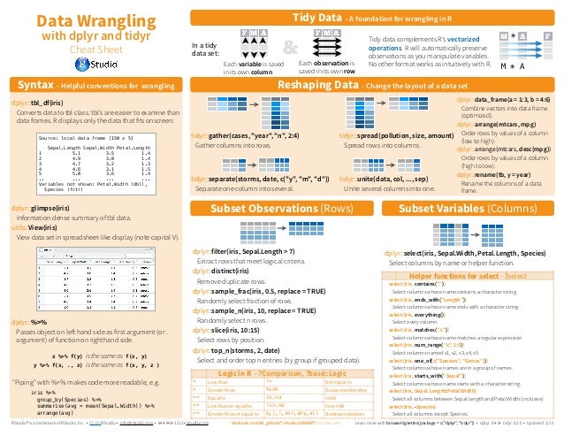
H - Reshaping with pivot_longer() and pivot_wider()
Remember the CD4_wide dataframe you created before? Currently it is in the wide format, where each row is a patient, where key data (different CD4 T cell counts) are in different columns like this:
# Data is in a 'wide' format
CD4_wide
# A tibble: 2,139 x 5
pidnum arms cd40 cd420 cd496
<dbl> <dbl> <dbl> <dbl> <dbl>
1 10056 2 422 477 660
2 10059 3 162 218 NA
3 10089 3 326 274 122
4 10093 3 287 394 NA
5 10124 0 504 353 660
6 10140 1 235 339 264
7 10165 0 244 225 106
8 10190 0 401 366 453
9 10198 3 214 107 8
10 10229 0 221 132 NA
# … with 2,129 more rowsOur goal is to convert this data to a ‘long’ format, where each row represents a single CD4 T cell count for a specific patient, like this:
# This is the same data in 'long' format
CD4_long
# A tibble: 6,417 x 4
pidnum arms name value
<dbl> <dbl> <chr> <dbl>
1 10056 2 cd40 422
2 10056 2 cd420 477
3 10056 2 cd496 660
4 10059 3 cd40 162
5 10059 3 cd420 218
6 10059 3 cd496 NA
7 10089 3 cd40 326
8 10089 3 cd420 274
9 10089 3 cd496 122
10 10093 3 cd40 287
# … with 6,407 more rows- Using the
pivot_longer()function, create a new dataframe calledCD4_longthat shows theCD4_widedata in the ‘long’ format. To do this, use the following template.
CD4_long <- CD4_wide %>%
  pivot_longer(starts_with("XX"))
Print your
CD4_longdataframe! Do you now see that each row is a specific observation for a patient?Now use the
pivot_wider()function to bring the data back into the wide format!
CD4_long %>%
  pivot_wider(names_from = XX,
              values_from = XX)
I - Grouped aggregation
- Now, apply the
group_by()-summarize()idiom to theCD4_widedataset to calculate the average (mean()) CD4 T cell counts for the various treamentarms.
CD4_wide %>%
  group_by(XX) %>%
  summarize(XX = XX,
            XX = XX,
            XX = XX)
Handle the missing values by including
na.rm = TRUEin themean()functions.Use
n()to add another summary showing the number of cases per arm.Now try to calculate the same values, but using the
CD4_longdataset. How do you need to adjust the code?Finally, use
pivot_widerto change the format of the summarized results to the one obtained fromCD4_wide.
Datasets
| File | Rows | Columns |
|---|---|---|
| trial_act.csv | 2139 | 27 |
| trial_act_demo_fake.csv | 2139 | 3 |
trial_act.csv
First 5 rows of trial_act.csv
| pidnum | age | wtkg | hemo | homo | drugs | karnof | oprior | z30 | zprior | preanti | race | gender | str2 | strat | symptom | treat | offtrt | cd40 | cd420 | cd496 | r | cd80 | cd820 | cens | days | arms |
|---|---|---|---|---|---|---|---|---|---|---|---|---|---|---|---|---|---|---|---|---|---|---|---|---|---|---|
| 10056 | 48 | 89.8 | 0 | 0 | 0 | 100 | 0 | 0 | 1 | 0 | 0 | 0 | 0 | 1 | 0 | 1 | 0 | 422 | 477 | 660 | 1 | 566 | 324 | 0 | 948 | 2 |
| 10059 | 61 | 49.4 | 0 | 0 | 0 | 90 | 0 | 1 | 1 | 895 | 0 | 0 | 1 | 3 | 0 | 1 | 0 | 162 | 218 | NA | 0 | 392 | 564 | 1 | 1002 | 3 |
| 10089 | 45 | 88.5 | 0 | 1 | 1 | 90 | 0 | 1 | 1 | 707 | 0 | 1 | 1 | 3 | 0 | 1 | 1 | 326 | 274 | 122 | 1 | 2063 | 1893 | 0 | 961 | 3 |
| 10093 | 47 | 85.3 | 0 | 1 | 0 | 100 | 0 | 1 | 1 | 1399 | 0 | 1 | 1 | 3 | 0 | 1 | 0 | 287 | 394 | NA | 0 | 1590 | 966 | 0 | 1166 | 3 |
| 10124 | 43 | 66.7 | 0 | 1 | 0 | 100 | 0 | 1 | 1 | 1352 | 0 | 1 | 1 | 3 | 0 | 0 | 0 | 504 | 353 | 660 | 1 | 870 | 782 | 0 | 1090 | 0 |
The trial_act.csv data set contains a randomized clinical trial to compare monotherapy with zidovudine or didanosine with combination therapy with zidovudine and didanosine or zidovudine and zalcitabine in adults infected with the human immunodeficiency virus type I whose CD4 T cell counts were between 200 and 500 per cubic millimeter.
| Name | Description |
|---|---|
| pidnum | patient’s ID number |
| age | age in years at baseline |
| wtkg | weight in kg at baseline |
| hemo | hemophilia (0=no, 1=yes) |
| homo | homosexual activity (0=no, 1=yes) |
| drugs | history of intravenous drug use (0=no, 1=yes) |
| karnof | Karnofsky score (on a scale of 0-100) |
| oprior | non-zidovudine antiretroviral therapy prior to initiation of study treatment (0=no, 1=yes) |
| z30 | zidovudine use in the 30 days prior to treatment initiation (0=no, 1=yes) |
| zprior | zidovudine use prior to treatment initiation (0=no, 1=yes) |
| preanti | number of days of previously received antiretroviral therapy |
| race | race (0=white, 1=non-white) |
| gender | gender (0=female, 1=male) |
| str2 | antiretroviral history (0=naive, 1=experienced) |
| strat | antiretroviral history stratification (1=’antiretroviral naive’, 2=’> 1 but ≤ 52 weeks of prior antiretroviral therapy’, 3=’> 52 weeks’) |
| symptom | symptomatic indicator (0=asymptomatic, 1=symptomatic) |
| treat | treatment indicator (0=zidovudine only, 1=other therapies) |
| offtrt | indicator of off-treatment before 96±5 weeks (0=no,1=yes) |
| cd40 | CD4 T cell count at baseline |
| cd420 | CD4 T cell count at 20±5 weeks |
| cd496 | CD4 T cell count at 96±5 weeks (=NA if missing) |
| r | missing CD4 T cell count at 96±5 weeks (0=missing, 1=observed) |
| cd80 | CD8 T cell count at baseline |
| cd820 | CD8 T cell count at 20±5 weeks |
| cens | indicator of observing the event in days |
| days | number of days until the first occurrence of: (i) a decline in CD4 T cell count of at least 50 (ii) an event indicating progression to AIDS, or (iii) death. |
| arms | treatment arm (0=zidovudine, 1=zidovudine and didanosine, 2=zidovudine and zalcitabine, 3=didanosine). |
trial_act_demo_fake.csv
First 5 rows of trial_act_demo_fake.csv
| pidnum | exercise | education |
|---|---|---|
| 10931 | 4 | HS |
| 11971 | 1 | <HS |
| 330244 | 1 | HS |
| 270879 | 1 | BA |
| 11435 | 0 | <HS |
The trial_act_demo_fake.csv data set contains fake demogrpahic information corresponding to the patients in trial_act.csv
| Name | Description |
|---|---|
| pidnum | patient’s ID number |
| exercise | the number of days per week that the patient exercises |
| education | the patient’s education level |
Functions
Packages
| Package | Installation |
|---|---|
tidyverse |
install.packages("tidyverse") |
Functions
| Function | Package | Description |
|---|---|---|
rename() |
dplyr |
Rename columns |
select() |
dplyr |
Select columns based on name or index |
filter() |
dplyr |
Select rows based on some logical criteria |
arrange() |
dplyr |
Sort rows |
mutate() |
dplyr |
Add new columns |
case_when() |
dplyr |
Recode values of a column |
group_by(), summarise() |
dplyr |
Group data and then calculate summary statistics |
left_join() |
dplyr |
Combine multiple data sets using a key column |
spread() |
tidyr |
Convert long data to wide format - from rows to columns |
gather() |
tidyr |
Convert wide data to long format - from columns to rows |
Resources
dplyr vignette
See https://cran.r-project.org/web/packages/dplyr/vignettes/dplyr.html for the full dplyr vignette with lots of wrangling tips and tricks.
Cheatsheets
from R Studio